What drives prices up?

There is common understanding in Australia that FHBs are one of the most important house price drivers. Is this really true?

Let's see what data shows:

Australia Property Investor/FHB market share vs. house prices

It is clear from the chart that there is a weak correlation between FHBs market share and house prices. For most of the time these two series were heading into opposite direction (correlation is slightly negative). On the other hand, property investors (PI) market share is very strongly correlated with house prices. This, of course, does not imply direct causation so we need more information. Just recently, US FED published report* that claims increase in property investors market share was the most important factor that created housing bubble in USA. Lower lending standards attracted large number of highly leveraged investors ready to take big mortgages with expectation of big and quick capital gains. They increased demand and drove prices up. FHBs and upgraders got squeezed and forced to pay ever increasing prices. Increasing prices attracted more investors and feedback started its own life independent of real demand or realistic future prospects. It's almost irrelevant what initiates the feedback loop; once started abundant and easy credit is only thing needed for growth.

According to FED property investor market share in bubble states increased from less than 25% in 2000 to almost 45% in 2006. Similar rise is property investors was recorded in Australia as a whole. In some areas (SE Qld, inner capital cities, ...) significantly higher percentage of investors entered property market and drove house prices by increasing debt to extreme levels. It is hard to imagine this trend to continue for long because of huge debt already accumulated. Once prices stop growing, property investors begin to sell because quick capital gain expectations are gone while big repayment bills continue to arrive every month. Most of highly leveraged and negatively geared investors cannot afford to hold for long without quick capital gain expectations.

Looks like same forces created housing bubbles in USA and Australia. Other minor factors made bubble extents and timings slightly different but core cause for rise and fall seem to be the same.


* http://www.ny.frb.org/research/staff_reports/sr514.pdf

Australian House Price Trend

There have been discussions that house prices cannot remain flat in “real” CPI adjusted terms because we are earn much more in “real” terms today that few decades ago. I agree that CPI adjusted prices should not be flat because CPI adjustment does not reflect standard of living improvements over time. House prices should follow more realistic measures of our improved wellbeing.

Chart 1 shows house prices in “real” (CPI adjusted) terms as well as growth of our real per capita GDP and per household GDP. These measures are one of few only with long historical series that could be used for price “trend” estimation.



Chart 1 "Real" House Prices vs. "Real" per Capita and Household GDP



Real per capita GDP is good measure because real GDP by itself ignores the fact that more than twice as many people contribute to GDP today compared to 50 years ago. On the other hand, houses are asset needed and owned by households, not the individual persons. In addition, number of homes is closely following number of households. For these reasons, real GDP per households seems to be better measure of the increased ability of households to spend money on home.

From the chart you may see that “real” (CPI adjusted) house prices followed real GDP per household with only few smaller property bubble events in mid 70s and late 80s. Prices returned toward the real GDP per household trend soon after. Since late 90s, house prices significantly deviated from real GDP per household trend. This deviation is strong indication that we are currently experiencing big housing bubble that is not supported by fundamentals.

This chart could give us a feel how much our homes are overvalued - inflated beyond historical and fundamental trend and what level of correction we may expect in near to mid future. Correction may happen with slow deflation in real terms or quick crush. It could be even combination like it was in 1990s when prices fell quickly by 10% in “real” terms and than stagnated while real GDP per household increased.

References:

1. ABS Australian National Accounts

2. ABS Australian Demographic Statistics

3. Stapledon

4. ABS House Price Indexes

Cost of Mortgage vs. Interest Rates

“New era of low interest rates” is often quoted as one of the main reasons for house price growth during 2000s. The argument claims that low interest rates reduce financing cost allowing house prices to increase for the financing cost reduction. This argument sounds very intuitive and as such it’s not questioned by many. So, let’s see how interest rates affect real (CPI adjusted) cost of house purchase.

First of all we should check relation between CPI and mortgage interest rates. This relation will significantly affect real cost of mortgage. On Chart 1, we may see strong correlation between the two but we should also notice that ratio between mortgage interest rate and CPI is decreasing as CPI is getting higher. In other words the lower the CPI - banks are charging higher margin. This means that the lower CPI, the more (in real terms) mortgage holder pays to bank over the life time of the mortgage.

Chart 1 - CPI and Standard Variable Bank Mortgage Rate

To calculate cost of mortgage financing we developed Mortgage Interest Rate to CPI ratio - see Chart 2.

Chart 2 - Annual CPI and Standard Variable Mortgage Interest Rate to CPI Ratio 

From the chart we may clearly see that the lower CPI the higher ratio. During the low interest ratio periods mortgage is much more expensive relative to cost of funding. This relation can be expressed in form of chart  based on historic data - see chart 3.

Chart 3 - Standard Variable Mortgage Rate to CPI ratio vs. CPI

When CPI is low banks are charging relatively (to CPI) high interest rates; on the other hand when CPI is extremely high banks charge less that CPI (they lose money). This combined with the fact that high inflation quickly reduces principal, should make us think that in real terms high CPI and higher mortgage rates could be better deal for mortgage holders. Chart 4 shows total cost of mortgage in CPI adjusted terms for 30 years 90% LVR loan for a given CPI and calculated interest rate based oh historic relation. Cost is calculated by assuming that CPI and interest rates remain the same over the entire period of the mortgage. This assumption is used to simulate cost dependency on low vs. high interest rate "eras" - argument used by people who claim that low Interest Rates (CPI) makes house purchase financing cheaper and house prices higher.

Chart 4 - Total Real Mortgage Cost Index (30 year)

Chart 4 shows that real cost of mortgage is significantly lower during periods of very high interest rates (high CPI). The reason for this is the fact that loan principal gets quickly eaten by inflation, and mortgage repayments quickly drop relative to income and other costs. It is also clear from the chart that cost of mortgage is relatively constant for periods when CPI is between 2 and 9%. So there are no reductions in total cost of financing house purchase between periods with moderate inflation (CPI 7-8%) e.g. during 1980s and periods with lower inflation (CPI ~3%) e.g. during 2000s.

Many people sell home before the end of the mortgage term so let's check what is the cost of mortgage for the first 10 years of 30 year mortgage - Chart 5. This period is selected because most of PPOR properties are held for at least 10 years before sale.

Chart 5 - Real Mortgage Cost After the First 10 years

As expected, cost of financing during first 10 years is higher for high interest rate mortgages, but unexpectedly for very high CPI periods cost decreases significantly. Cost of financing for the first 10 years is the highest for CPI around 8%. The difference between maximum cost for CPI of 7-8% (during 1980s) and cost for CPI of 3% (during 2000s) is around 20%. So if majority of people hold PPOR property for 10 years, cost of financing reduction due to low rates could drive prices 20% in real terms between 1980s to 2000s. 

Lower interest rates also make repayments during first few years lower compared to income. This means that people can take much higher debt during low inflation periods if repayment as percentage of vs. income lending criteria remains the same.  

Chart 6 - Real Mortgage Cost Index

From Chart 6. we may see that remaining part of a mortgage after 10 years is significantly lower during periods of higher inflation. This means that people much quickly repay their debts than what is the case for low inflation periods.

We may conclude that total cost of financing has general trend of falling with CPI and interest rate increase and it is fairly constant for low (3%) and medium (7%) CPI periods. As such, it cannot be used to justify real house price increase. Short term (10 year) mortgage cost is slightly lower during low inflation periods and could be used to justify house price increase of around 20%.

Most importantly lower interest rates make initial repayments lower allowing people to take much larger debt relative to income and that could be one of the key drivers (combined with lower LVRs) for house price increase during 2000s.  

Low rates (CPI) allow people to take much more debt relative to income, they make mortgages more expensive over the mortgage life and they keep people in high debt for much longer period by keeping loan principal high. This is not only the key reasons why our (spending) economy is suffering but also the reason why it will not be able to recover anytime soon (if CPI remains on these levels). 

To avoid this debt trap caused by low CPI and mortgage rates, banks could adjust lending criteria and take into account CPI levels. They had to reduce maximum LVR and maximum repayment relative to income to offset low interest rate trap. During 2000s, not only that we let low rates to do  the damage but also our banks increased LVR and maximum repayments relative to income, creating huge debt problem that will cause economic pain for extended period.

"Predictions" by Google Insight

There are a lot of discussions about timing of Australian property bubble. It is impossible to predict timing of events such is bubble burst but to make this interesting I checked Google Insights for Search to see whether search for “property/housing bubble” can be used for predictions.

Findings are quite surprising – see charts.

Charts 1 House prices and Google Searches - Ireland

Charts 2 House prices and Google Searches - Spain

Charts 3 House prices and Google Searches - UK

Charts 4 House prices and Google Searches - USA

From charts you may notice that peak search for phrases “property/housing bubble” happened 2-3 quarters before bubbles bursted in these countries. This is very interesting and IMHO probably tells a lot about the fact that sentiment plays very important role in market movements. What is surprising to me is the fact that search for bubble information drops before bubble bursts and stays lower when most equity wealth disappears and most of people lose their homes.    

Now, lets take a look at Australian search for "housing bubble"

Charts 5 Google Search "housing bubble" - Australia

Search for "housing bubble" peaked in November 2010 - 8 months ago. Based on Google Insight for Search information for other countries with similar housing bubbles, Australian housing market is just at the turning point and future doesn't look good. Data that is being published these days suggests that Google might be right.

BTW. UK market also doesn't look promising after slight recovery in 2008, "search sentiment" is up again.

Will RBA save the housing?

There is a lot discussion around about RBA's ability to stop house price fall using rate cuts). The argument for this is 2008-2009 period when allegedly RBA stoped price fall and government even inflated prices using FHBG. Second argument people use is that USA had fixed rate mortgages that stoped similar policy work there. Other people use UK example to show that lower rates cannot stop but rather slowdown the price fall. Surprisingly to many, I think our situation is more similar to Irish.

In 2006-07 when bubble bursted in USA situation was in many ways different than in Australia year after when GFC broke out. I would agree that RBA rate cuts in 2008 saved house prices but the timing of cuts was different from what we may expect today. Reason for RBA cuts in 2008 was not falling house prices, but outbreak of GFC. Rate cuts were just on time to save house prices that just started falling few months before rate cuts. In addition, Australian sentiment about house prices in 2008 was completely different. People believed that house price fall was caused by external disturbance – GFC, and that after disturbance is removed housing will continue growth.

Today, there are not so many similarities with our situation in 2008, but there are many similarities with conditions in other countries at that time. Surprisingly Ireland is in my focus. House prices started to fall in Ireland but interest rates were on rise some time after (five rises after the peak price).  Reasons for this are EURO and Ireland’s lack of Interest rate control. This situation looks completely different than ours but the core reason looks very similar to RBA inability to respond to falling house prices. ECB had to deal with two speed economy in Eurozone. In 2007 debt driven economies of PIIGS were heading into recession (or were already there as Ireland) while some other parts of Eurozone was doing very well. ECB was not able to respond to rising inflation in some countries and falling prices in Ireland at the same time.

Our situation today is quite similar. We also have two speed economy that prevents RBA to use rates as a response on house prices only. Under current conditions and falling house prices at current rates it is unlikely that will see rate cuts soon - before economy starts feeling the pain on larger scale. Global inflation, instead deflation is this time around making RBA job even harder. This environment will force RBA make decisions in ECB rather than the FED style.

Even if RBA decides to respond on housing only while risking inflation, as FED did, rate cuts will not happen any time soon. FED started cutting rates over a year after bubble bursted (prices started to fall). By that time tipping point was already reached. Rate cuts combined with FHBG somewhat helped house prices in USA to stop falling but almost a year after first cuts.

Sentiment is one of the main drivers of bubbles whether up or down. This time, housing crush is just our own; nobody can blame external forces for crush or hope that everything will be fine if external problem gets solved. People are aware that house price fall is result of a bubble that we inflated. They know that if rates get cut again that will be just temporarily relief.

Even an unlikely scenario (RBA cuts rates now to help house prices) would just prolong what must happened – significant price correction. RBA is well aware of this and they are trying to make correction slow to minimize effect on the economy. Their ultimate goal is stagnation over long period (slow fall in real terms). I don’t believe they will be able to achieve that because of two speed economy we have. Our housing is more like PIIGS’s debt while our mining is German export. Our rates will stay the same (or even go up a little bit) for some time, and when finally RBA cuts them it will be too little too late.

RENT vs. BUY CALCULATOR (Australia)

Most of the existing free online BUY vs. RENT calculators are not adjusted for Australian market (like the famous NYT calculator), or they provide just a few available settings and options. I tried to a make calculator that will give people opportunity to enter certain assumptions about inflation, house price growth, IR, returns … for 5 years periods and get some meaningful results. I also tried to include as many variables as useful. There are “BUY NOW vs. RENT” and “BUY NOW vs. BUY in 10 YEARS” comparisons that may be useful under current housing conditions (expected house price stagnation or fall).

Calculator provides few different results: It calculates total wealth after the same amount of money is being "spent" using different options. In addition, it calculates number of years after which “BUY NOW” option is financially better off. Or in other words: How long a person has to live in that particular house to be better off financially? If for any reason (even upgrade), buyer sells the home before, he would be better off by renting all the time.
I also added an option for renters to rent cheaper (smaller) home during first 5 years – this could be useful for young families with no children.

There are two sheets in this file: CALC sheet enables user to enter data and assumptions. It also gives basic results: “wealth after 45 years” and “number of years after BUY NOW option is better off financially”. DETAILS sheet provides all calculations and results for each year and each option.

Here is link for xls file download: BUY vs. RENT Calculator 

You need to have spreadsheet viewer or editor installed on your computer to be able to use this file. People who don’t have spreadsheet viewer or prefer not to download file, may use a link to web based spreadsheet version of calculator. It will open file in Google doc frame. You do not need to have Google account to open and use this calculator.

WEB-BASED BUY vs. RENT Spreadsheet CALCULATOR

You are free to share calculator links but please do not distribute calculator as downloaded spreadsheet file because any future fix or modification will not affect downloaded file.

Assumptions: Immediate buyer buys home with current savings; renter saves that money and difference between rent and cost of owning a home. After 10 years, "late buyer" buys the same home (for future price), giving 90% of his savings as deposit. During periods when renter or late buyer spends more on housing, immediate buyer saves the difference. Rent and other costs of owning (strata, council etc. grow with CPI). Calculator assumes that renter moves once in 3 years. FHBG is assumed to be nominally the same in 10 years. If you have questions about other assumptions not mentioned please contact me and I will provide you requested assumptions.

Calculator uses assumptions entered by user, default assumptions or calculator results should not be taken as investment advice. I don't have time to fully test it so there might be some errors. I would appreciate any help in finding errors. Please post comment on the blog or contact me on rave.swei@yahoo.com if you find any significant error that needs to be fixed.

Popping Timing

Many people ask me recently when prices will fall; when it will hit banks; when unemployment will go up ...

It is impossible to predict timing of a such event. To help us understand timescale of the process I created a charts that show timings of the bubble bursts in Ireland and USA.

USA and Ireland Bubble Deflation Timing

On the chart you may see that house prices started deflating very early (July 2006 in USA and July 2006 for Ireland and few months later in Dublin). At the beginning price correction was very slow. It took almost a year and a half in USA and even longer in Ireland to drop 10% from the peak. It took two years for majority of people to realize that something is very wrong. Even the most involved people like FED chairman Ben Bernanke*, two years after process started were not aware (or willing to admit) that country is facing serious problem caused bu housing bubble burst).

It is even more interesting to see changes in major economic parameters during this period. Prices started falling while unemployment was very low. Even after correction started unemployment continued to be very low and even dropped in USA. It took more than a year after prices started to fall for unemployment to start rising and more than 3 years to reach maximum. GDP growth was very healthy at the moment prices started to fall and remained healthy for a year or more after that.

It is also interesting to see that house prices started falling while interest rates were going up. Than prices continued to fall while rates were stable but fall accelerated with interest rate cuts. Credit was available and  inflation was at normal level for the period; business and/or consumer confidence was very high. Maybe the most revealing part is saving rate. Prices started falling at the peak of the saving as a percentage of GDP. 

Consequences of both bursts were severe: deep recession, high unemployment, deflation, credit squeeze, zero interest rates, drop in saving rates and confidence.

If someone was presented with the charts up to the point of house price burst, he/she would likely say that future is bright because all economic parameters were good. In reality things were much different, high level of debt and long period of misallocation of investments into housing caused one of the most severe recessions in history. Low unemployment, high saving rates, high confidence, GDP growth and high interest rates that in theory should enable central bank to react were not enough to prevent the worst.

What will be timeline of the Australian housing bubble burst is impossible to say. If we can learn anything from this data, that should be caution. At the beginning it always looks harmless - ordinary cycle price correction; nothing more than that. It quickly develops in galloping destruction of the economy and no action form central bank or government is able to stop it. 

* Ben Bernanke (June 10, 2008) “The risk that the economy has entered a substantial downturn appears to have diminished over the past month or so.” 

Sources:

- http://www.tradingeconomics.com

- S&P/Case-Shiller Home Price Indices

- Economic and Social Research Institute (ESRI), Dublin, Ireland

Construction Response on Rising House Prices

In addition to Rates of Construction and Rates of Occupancy that we presented in our last paper, we want to research construction industry activities. As a measure of a construction industry activities we will use construction employment data for the 15 years period (1996-2010) for Australian and USA states and period 1998-2010 for a few countries (we could not find data for Ireland and Spain prior to 1998). We calculated two numbers: Construction jobs as a percentage of total employment and corresponding Index. Sources of data are OECD, USA Bureau of Labour, Federal Reserve Bank of St. Louis and ABS.

Chart 1 – Construction Jobs in Australia

First we want to show historical change of construction jobs in Australia. Data is available for a period 1984-2010. From the chart we may clearly see increase in the construction jobs during the price increase since 2000.

Chart 2 – Construction Jobs as % of Total

  

From this chart and additional data from Ireland we may see that Ireland as well as Spain have historically higher percentage of construction workers. This may be caused by different construction methods used in different countries. These methods are not equally labour intensive (full-brick and concrete in Europe, veneer brick and wood in Australia and USA). To somehow offset for these fundamental differences we created Index with the 1998 as a base year. This way we may see relative changes of the construction activities over this period.

Chart 3 - Construction Jobs as % of Total - Index

From this chart it is clear that Ireland had huge construction boom from the beginnings of 2000s with the very strong upswing in 2004. This boom lasted until crash of 2007 when construction industry collapsed below 1998 levels. Spain had much lower increase of the construction job share; it grew to 130% of 1998 levels and than dropped significantly (notice on Chart 2 that after big fall Spain percentage is still high compared to USA and UK peak levels). Australian construction jobs also grew significantly, by 2008 almost recording the same increase as Spain two years before. Australian construction jobs are still very high compared to pre-bubble period in other countries.

State Comparison

Most of the construction activities are residential, but not all. We tried to find data that shows percentage of total construction employment that is related to residential construction. We were able to find some data, in our opinion enough to show that significant majority of jobs are related to the residential construction.

Table 1 – Percentage of the Residential Construction Jobs

Chart 4 - Heavy and Civil Construction Jobs

From Table 1 we may see that around 25% of all construction jobs in USA are not directly related to residential activities and around 15% in Australia – slightly lower percentage in Australia. Chart 4 shows that non-building (mining and infrastructure) jobs fell during the same period. This clearly shows that most of the construction boom is related to residential building construction.

Chart 5 - Construction Jobs as % of Total (by state)

Chart 6 - Construction Jobs as % of Total (by state)

Charts 5 and 6 show construction job percentages for large Australian states (NSW, VIC, QLD, SA and WA) as well as some of the USA states used in previous analysis (CA, FL, AZ, NV and TX). We may notice that some states have significantly higher percentage in both countries. We speculate that this is consequence of large non-residential construction activities in these states (resource activities in WA and QLD and military/tourism activities in NV). Unfortunately we were not able to find adequate data to support this view.

In other states, growth was very similar over the period before the crush in USA. After USA percentages dropped in 2007 all Australian states grew even more, reaching highest levels during the period 2008-2010. 

Chart 6 - Construction Jobs as % of Total – Index (by state)

Chart 7 - Construction Jobs as % of Total – Index (by state)

On charts 6 and 7 we plotted construction job index for the same period. Please, notice that almost all USA states recorded smaller increase in construction job activities than Australian states. The only exception is California, that at the beginning of the period, was still recovering from housing bubble crash from early 90s. At that time California had by far the lowest percentage of construction jobs 4%, while the lowest in Australia was SA with 5.5%. SA recored the largest growth of the construction job sector that clearly corresponds to largest Rate of Construction we calculated in our previous paper. 

From all presented data we may conclude that Australian construction response to growing house prices was high relative to historical levels; it was lower than response in Ireland but very close to Spanish and significantly higher than response in USA or UK.

The response in Australian states was at least equally strong as responses in selected USA states (measured by construction employment). These USA states are currently facing huge oversupply of homes and collapsing construction industry. This just confirms our previous statements that Australia has large oversupply of homes build during the price bubble over the last decade. It also suggest potential for a big collapse of the residential construction industry that will certainly hurt overall economy.

Sources:

- Federal Reserve Bank of St. Louis Construction Employment by State

- 6291.0.55.003 - Labour Force, Australia, Detailed, Quarterly, Aug 2010

- OECD Statistics

- USA BOL Nongovernment distribution of wage and salary employment in construction by industry, 2000-2008

- ABC 8772.0 - Private Sector Construction Industry, Australia, 1996-97  ;  2002-2003

- Central Statistics Office Ireland - Index of Employment in Building and Construction

Australian Housing Shortage/Oversupply by State/Territory

Our previous paper showed that there is very likely to be oversupply of homes in Australia. Now we want to see where all that oversupply is located. We will make comparison between different states in Australia and add comparison with some of the states in USA that are well known for their housing bubbles followed by oversupply. This way we may get a feel about different supply/demand values compared to other areas with similar demographics.

We used data is available for all selected states and territories. Population growth and new dwelling construction data is used. There is no data available with detailed breakdown of new resident population for each state or territory. We also compared Australian states and territories with a couple of USA states that had large housing bubbles followed by price collapse and huge oversupplies of homes. We also included Texas, high population growth state that didn’t experienced housing bubble in last two decades, as an opposite reference.

USA is selected for comparison because of very similar demographics to Australia. Main supply/demand demographic measures such are household size and change in household size, median age, population over 65 and under 14, birth rate, dependency ratio, percentage of one person households, urban population growth etc) are very similar. For new construction data in Australia we used ABS New Dwelling Unit Commencements data.  For new construction data in USA we used New Private Housing Units Authorized by Building Permit provided by Federal Reserve Bank of St. Louis. Number of newly constructed dwellings for US is likely to be slightly lower because not all approvals are commenced. We used data for the most recent period from June 2000 to June 2010.

We calculated two simple measures that we call: Rate of Construction and Rate of Occupancy. Rate of Construction is a number that shows how many new housing units are constructed per every new resident. Rate of Occupancy is the inverse number that shows number of new residents per each newly constructed housing unit. After calculation we got a few surprising results:

Table 1. Rate of Construction and Occupancy

Chart 1. Rate of Construction (new dwellings per new resident)

Contrary to widespread belief, Queensland is the state with the lowest Rate of Construction in Australia (NT has even lower rate). South Australia, on the other hand, is the state with the highest Rate of Construction. Expectedly, high Rate of Construction is recorded in Victoria and ACT but surprisingly WA is ranked in lower half, followed by NSW, QLD and NT that had very low construction rate.

Even more surprising is comparison with housing bubble states in USA. South Australia has significantly higher Rate of Construction than any of the famous bubble states in USA. Victoria had very similar rate to hugely oversupplied Florida. NSW has higher Rate of Construction than Arizona, Nevada and almost 20% higher than California, state that is currently dealing with hundreds of thousands of empty homes. On the other hand, all Australian states have significantly lower rate than Texas, state with the large population growth but stable house prices with no housing reported shortage.

All this suggests that widespread beliefs about shortage/oversupply in Australia are wrong. Queensland is the state with the lowest Rate of Construction because its population grew much faster. Almost all Australian States built more dwellings than bubble states in USA that are currently dealing with huge numbers of empty homes. It is also important to notice that at the peak of the price bubble, almost all of these USA states were considered to have a shortage. That was proven to be wrong after bubble bursted and speculative demand fell.

It is very unlikely that there is any housing shortage (on state level) in Australia, but if there was one Queensland and NT were the most likely to have it. This is very surprising because Queensland is the state that will be pointed out as oversupplied state by most of Australians.

Recent data shows that low construction state’s (Queensland and Western Australia) housing markets are falling, with unsold stock growing and oversupply becoming apparent. If these states with relatively low Rate of Construction are facing oversupply problem, we may expect to be followed by even more oversupplied states like Victoria, South Australia, Tasmania and New South Wales.

References:

- ABS 3101.0 - Australian Demographic Statistics, Jun 2000, June 2010

- ABS 8750.0 Dwelling Unit Commencements, Australia, Preliminary Dec 2010

- United States Census Bureau - Census Data 2000 and 2010

- Federal Reserve Bank of St. Louis – New Private Housing Units Authorized By Building Permit

Australian Residential Housing Demand and Supply

By raveswei

This document will try to research one of the most controversial housing issues in Australia – supply/demand issue. Many times we heard arguments that Australia is facing a chronic shortage or that price boom is not followed by supply response. At the same time, some people claim that we have oversupply of homes for decades. In this document we will try to estimate residential demand and supply in recent years. We will focus on demand/supply for dwellings used as primary residence. This is very complex issue because of many unknowns and limited data. We will try to make assumptions that will favour shortage argument. Data for Australian cities are not available so this document will focus on all of Australia.

Document will be organized in the following order: In a first few sections, we will go through the supply and demand calculations for one particular year (2007-08), showing the data sources and methodology. Later we will provide data for a period 1995-2010 calculated using the same data sources and methodology. At the end we will give a conclusion.

All raw data used is provided by ABS or Department of Immigration.

DEMAND

Estimation of the demand for housing is not easy task. Demand is driven by many factors, but two of them are the most important: population growth and household demographics change. Population growth has two components: natural increase and net overseas migration.

Migration

Immigration is one of the most important drivers of the housing demand in Australia. Both immigration components (permanent and temporary), increase housing demand in the short term and should be included in calculations. In 2007-08 there was 277 000 net migrants (number of immigrants minus number of emigrants). There was 149 400 permanent arrivals and 76 900 permanent departures. Out of this number there was almost 38 400 “family immigrants” - large majority of them (80%) being partners and children. It is a reasonable to assume that these immigrants do not contribute to the new housing demand (do not create new households) in the first year after arrival. On longer run some of them will require new homes but that demand will be included in the demand calculation that uses households size changes.

Because of the similar demographics among permanent immigrants and emigrants we may assume that dwellings previously used by emigrants are adequate for the same number of immigrants. This assumption is based on similar age, similar proportion of children, occupation... This leaves only 38 400 permanent immigrants in need for a new home. After taking into account fact that around 15% of them are dependent children, assumption of household size of 2 persons is well on the safe side. In 2007-08 these immigrants created demand for 19 200 dwellings.

Net number of temporary, long term visitor, immigrants in 2007-08 was 205 200 with majority of them being foreign students and WHMs. Around 73% of all long term visitors (long term visitors include following groups: temporary workers, students and WHMs) 149 800 were students and WHMs, majority of them being students from China and India. This group of a temporary immigrants add less demand for new housing than the general immigration population. Some of WHMs stay in hostels and budget hotels, not adding any demand for residential housing. Estimation of foreign student and WHM demand for residential housing is not strait forward, but based on student living habits we think that assumption that average student household size of 2.5 is well on the safe side. There are many student living arrangements that involve 3, 4 or more students sharing the same dwelling. This created demand for 59 900 dwellings.
The rest of temporary immigrants (55 400) are workers and their families. We will use household size of 2 to be on safe side. It is very likely that workers who arrived with families live in larger households. It is also likely that some of the single workers share dwelling with other single persons. They created demand for 27 700 dwellings.

References:

ABS 3412.0 Migration 1995-2008

- Department of Immigration and Citizenship – Migration Program Statistics http://www.immi.gov.au/media/statistics/statistical-info/visa-grants/migrant.htm

- Department of Immigration and Citizenship – Fact Sheet – Permanent Arrivals and Departures - http://www.immi.gov.au/media/fact-sheets/05emigration_1.htm

- Department of Immigration and Citizenship – Population flows: Immigration aspects 2000-2009

- Department of Immigration and Citizenship - Settler Arrivals 2001 – 2010

- Department of Immigration and Citizenship - Immigration in Brief 2000

Natural population increase

There was 289 500 births and 140 700 deaths in 2007-08. This makes natural population growth of 148 800. Births do not directly increase the demand for new dwellings, but they affect household size and distribution. The best way to estimate internal demand for new housing is to determine housing demands generated by demographic changes and natural population increase.

Unfortunately the number of households is available only for census years and the number of migrant households is not available at all. Instead we will use following formula:  

This formula includes new housing demand from natural increase and demand from household demographic changes. Household size change includes all of previous population changes (including divorces, marriages, new household creation, previous migration …). Good way to estimate demand from household changes is to use household size number.

Household size change can be calculated using the closest two census data with assumption that change during short period between two censuses is linear.

It is interesting to notice that according to census based data, household size slightly increased between 2001 and 2006. For the years after 2006 we will use new ABS household projections (Series II) that projects household size shrinking in following decades. This numbers are very likely to be underestimated because two previous ABS projections were wrong (ie. in 2001 ABS projected household size to shrink to 2.5 in 2006, instead household size increased by 0.01).

In year 2007-2008 there was 21 432 000 Australian residents, the projected household size of 2.62 and projected household size change of -0.38%. This data gives additional demand from natural increase of population was 56 800. Demand generated by household shrinking in 2007-08 was 33 600. Combined internal demand for new dwellings was 90 400.

Total demand for additional dwellings in 2007-2008 was 198 900. Please notice that this number is much larger that estimates provided by other people who use population increase divided by average household size (163 000).

References:

- ABS 3236.0 Household and Family Projections (1996-2001-2006)

- ABS 1301.0 Year Book Australia 1995-2010

- ABS 3222.0 - Population Projections, Australia, 2006 to 2101

- ABS Census Data (1996-2001-2006)

SUPPLY

There are two components of a housing supply. The first and the obvious one, is new dwelling construction supply. Second component of housing supply is made of vacant dwellings after resident’s death. In this section we will try to estimate these numbers.

New Construction

For the new construction supply we will use ABS Number of dwelling units Commenced. This number is slightly lower than Number of New dwelling units Approval, what put us on the safer side because not all aproved units are built.

In 2007-2008 there were 158 500 new unit commencements. To get more realistic number of the new residential dwelling supply we have to subtract number of dwellings that were demolished or replaced during the same period. To estimate this number we will use available data from Queensland. During 5 year period (2001-2006) around 1% of housing stock in Brisbane LGA was replaced or demolished. The same report estimates replacement levels of 0.5% in Gold Coast City, 0.25% in other urban LGAs, and 0.1% in the rest of Queensland. To be well on the safe side we will use 1% replacement level over 5 year period for whole Australia. This estimate is likely to be well above the real number because not all of the new construction is done in central LGAs. Using the estimate that housing stock was 1.06 times higher than number of households we got 17 300 demolished or replaced dwellings in 2007-08.

The total number of newly constructed residential dwellings in 2007-08 was 141 200. Some of these homes were holiday homes not available for new residents, so we have to subtract holiday homes from the total number. We will use generous estimate that around 4% of all new dwellings are holiday homes. That makes 5650 of new dwellings holiday homes. So the total number of new dwellings available for primary residence in 2007-08 was 135 500.

References:

- ABS 8750.0 - Dwelling Unit Commencements

- Queensland Department of Local Government, Planning, Sport and Recreation - Household projections, Queensland Local Government Areas 2007- Appendix A

Other Supply

Single person households create housing supply after the resident dies. In this section we will try to estimate number of dwellings made vacant after resident death.

Huge majority of Australians who die are old persons, 80% of persons who died in 2008 were 65+ at the time of death. There were around 140 700 deaths in that year. According to ABS data, in 1996 38% of population 65+ were living alone. This number is projected to increase by 84% in next 25 years. This gives us 50.5% of 65+ people living alone in 2007-2008; to be safely on the conservative side we will use 5% lower estimate - 45.5%. There are also some living alone persons under age of 65 who died but to be on the safe side we will not include them in our calculation.

After taking into account all this we may say that more than 51 000 dwellings are made available by the resident death in 2007-08. This number significantly adds to the supply side and it is often neglected by other authors. Combined, new construction supply and supply from homes vacant after the resident death makes total supply in 2007-08 of 186 500 homes available for new residents.

References:

- ABS 3302.0 – Deaths 1995-2010

- ABS 1301.0 Year Book Australia 1995-2010

- ABS 3236.0 Household and Family Projections (1996-2021, 2001-2026)

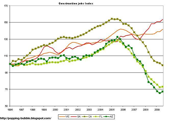
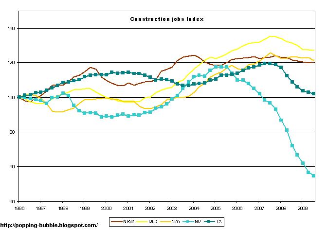
TRENDS

In this section we present results that we calculated using the same methodology we used for year 2007-2008. Some data (household size) between censuses is estimated using linear progression. This is likely to be a good estimate because of the nature of data set and short period between two censuses. Table 1 shows estimated demand and supply for period between year 1994-1995 and 2009-2010.

Table 1. Supply and Demand for residential dwellings in Australia

Chart 1. Supply and Demand for residential dwellings in Australia

CONCLUSION

By looking at the results we may see that Australia is facing huge oversupply of residential dwellings. Since 1995, there were only two years of a construction undersupply (2008 and 2009) driven by huge immigration numbers. During the years before that, Australia was building the similar number of new homes while immigration and population increase was half or even third of the 2008 or 2009 levels. After 15 years of construction, almost 950 000 dwellings that now do not have primary resident were built. That is around 10% of total housing stock. This means that around 38% of newly constructed dwellings during this period were oversupply (not used as primary resident or holiday home).

It may look very strange that such a huge oversupply is not easily visible. The reason for this, in our opinion, is the fact that market demand for housing was huge and in large part driven by investors interested in capital gain. Similar market behaviour was recorded in some parts of USA and Europe recently. In all these places, during the period before market crush, many reports were warning of a housing shortage, just to discover huge real oversupply after bubble bursted.  

This is an estimated number, intentionally biased toward the undersupply side and as such, it is good enough to shows that there is significant real oversupply of homes in Australia. Situation in a particular city may be slightly different but after taking into account that combined capital city population did not grow faster than general population we may say that estimates are good for most of the cities. Some of capital cities (Sydney, Hobart, and Adelaide) had slower that the average population growth. Same cities also recorded lower construction activity and slightly larger mortality rates among older population. In addition, Sydney and Melbourne population increase was mostly driven by student population that demands less housing than natural increase or other immigrants. Some of the areas with high construction activity (Gold Coast, SE and North Queensland, Mandurah) were also fastest population growing areas in Australia.   

Huge real (primary residence) oversupply will significantly impact house prices in Australia in future. In the case of market slowdown, oversupply will flood the market driving prices down.  


Calculation table:
table.pdf